


Abstract
We report on the observation of fine-scale structure in the outer corona at solar maximum, using deep-exposure campaign data from the Solar Terrestrial Relations Observatory-A (STEREO-A)/COR2 coronagraph coupled with postprocessing to further reduce noise and thereby improve effective spatial resolution. The processed images reveal radial structure with high density contrast at all observable scales down to the optical limit of the instrument, giving the corona a "woodgrain" appearance. Inferred density varies by an order of magnitude on spatial scales of 50 Mm and follows an f−1 spatial spectrum. The variations belie the notion of a smooth outer corona. They are inconsistent with a well-defined "Alfvén surface," indicating instead a more nuanced "Alfvén zone"—a broad trans-Alfvénic region rather than a simple boundary. Intermittent compact structures are also present at all observable scales, forming a size spectrum with the familiar "Sheeley blobs" at the large-scale end. We use these structures to track overall flow and acceleration, finding that it is highly inhomogeneous and accelerates gradually out to the limit of the COR2 field of view. Lagged autocorrelation of the corona has an enigmatic dip around 10 R⊙, perhaps pointing to new phenomena near this altitude. These results point toward a highly complex outer corona with far more structure and local dynamics than has been apparent. We discuss the impact of these results on solar and solar-wind physics and what future studies and measurements are necessary to build upon them.
Export citation and abstract BibTeX RIS

Original content from this work may be used under the terms of the Creative Commons Attribution 3.0 licence. Any further distribution of this work must maintain attribution to the author(s) and the title of the work, journal citation and DOI.
1. Introduction
Direct imaging of the solar corona has a long and storied history. Eclipse observations date back centuries. In the 1930s, Bernard Lyot (1930, 1939) developed a technique to minimize the light diffracted from the edge of the entrance aperture. His impetus was to develop an instrument—the internally occulted coronagraph—to image the solar corona from the ground. That concept was extended to the externally occulted Lyot coronagraphs carried by spacecraft, for example, the Orbiting Solar Observatory-7 (OSO-7; Koomen et al. 1975), which operated from 1971 to 1974, and Skylab (MacQueen et al. 1974), which operated from 1973–1974. Although OSO-7 observed the first coronal mass ejection (CME), the quality of its secondary emission cathode (SEC)-Vidicon detector could not compare to the details in the CMEs observed with the film camera in the Skylab coronagraph. The P78-1 (Solwind) coronagraph (Michels et al. 1980), operating from 1979 to 1985, was a duplicate of the OSO-7 coronagraph, but was modified to record a full 256 × 256 pixel image of the corona out to 10 R⊙ in about 4.4 minutes, instead of 44 minutes. It was operated at a regular cadence and therefore was able to observe many CMEs (Howard et al. 1982; Webb & Howard 1994), including the "halo CME"—the first Earth-directed CME observed in white light (Howard et al. 1982). The Solar Maximum Mission coronagraph (MacQueen et al. 1980) observed the corona in 1980 and 1984–1989 out to 6 R⊙ in a "quadrant mode" that enabled CME detection with higher spatial resolution than previously; accomplishments included the discovery of the three-part CME (Illing & Hundhausen 1985).
Then in 1995, the era of the charge-coupled device (CCD) detector began. The Large Angle and Spectrometric Coronagraph (LASCO; Brueckner et al. 1995) was launched on the Solar and Heliospheric Observatory (SOHO; Domingo et al. 1995). The three LASCO coronagraphs each carried a 1024 × 1024 CCD, which had higher spatial and photometric resolution than the previous instruments and together imaged the corona out to 32 R⊙. The sensitivity improvements revealed an unanticipated level of variability along coronal structures, in both spatial and temporal scales, with clearly outflowing plasma mimicking the acceleration postulated for the solar wind (Sheeley et al. 1997).
Beginning in 2007, the five telescopes within the SECCHI suite (Howard et al. 2008) carried on the Solar Terrestrial Relations Observatory (STEREO) spacecraft (Kaiser et al. 2008) observed the heliosphere from the surface of the Sun to about 384 R⊙ and, for the first time, imaged the fluctuating solar wind beyond 30 RSun (Sheeley et al. 2008). In addition to CME imaging (e.g., Thernisien et al. 2009; Liewer et al. 2010; Poomvises et al. 2010; Mishra et al. 2015), the wide-field imagers in SECCHI have yielded important results on the structure of the solar wind itself, including observation of small-scale periodic density enhancements convected out with the solar wind (Viall et al. 2010; Rouillard et al. 2011). More recent analyses include measurements of the outer limits of the corona (DeForest et al. 2016) and observations of the nascent stages of a stream interaction region (SIR; Stenborg & Howard 2017). These works, in particular, highlight the importance of careful postprocessing to extract a meaningful signal that is present in the data but is not apparent with conventional coronagraphic background subtraction.
Coronal structure in both the HI-1 and COR2 (the inner heliospheric imager and the outer coronagraph, respectively) fields of view has highlighted the interplay between the effective spatial resolution of a measurement and the signal-to-noise ratio (S/N) of that measurement. The photometric noise level in a digital image or image sequence is scale dependent (e.g., Vaseghi 2006), because each pixel includes an independent sample of both the image data (which may be correlated between different locations in time and space) and the image noise (the dominant elements of which are uncorrelated across time and space). Averaging an image's value across samples reduces the photometric noise by a factor of  , where Nsamp is the approximate number of independent measurements drawn from the original image or sequence; but if a single image feature spans all Nsamp samples, then its signal strength is unchanged under averaging so that the averaging operation increases the S/N. Put another way, image features at large scales can be detected far more sensitively in a given data stream than image features at small scales. This effect is exacerbated, in the optically thin corona, by the importance of line-of-sight integration—which causes small coronal features to have brightnesses that scale approximately linearly with size. Thus, the S/N for detection of features with a length scale of L scales roughly as S/N ∼ L2 to S/N ∼ L1.5. The steeper slope corresponds to compact features such as blobs, with Nsamp ∼ L2, and the shallower slope corresponds to long linear features such as coronal striae, with Nsamp ∼ L. For each measurement, there is a length scale, Lmin, below which the typical S/N drops below unity. If Lmin is larger than the instrument's optical resolution, then it sets the effective resolution of the measurement. The effect is illustrated in Figure 1.
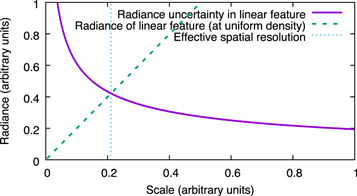
Figure 1. Photometric noise can limit spatial resolution. Photometric uncertainty grows as the feature scale decreases (to the left), while feature strength drops. Where the curves cross, S/N = 1. Smaller features are not detected, even if the instrument, in principle, resolves them.
Download figure:
Standard image High-resolution imageThe spatial resolution of essentially all spaceborne coronagraphic measurements to date, and those of COR2 in particular, have been limited by S/N effects rather than by instrument optics. This motivated us, in 2014, to run a "deep-field" campaign with the SECCHI/COR2 instrument, capturing the near-solar-maximum corona with the highest S/N possible to probe small, faint features in the corona (such as possible inbound jets and waves that might serve as markers of the Alfvén surface).
The 2014 campaign summed nominal 6 s COR2 exposure frames on board STEREO-A to form the equivalent of a 36 s unpolarized exposure, once every 5 minutes, over a 72 hr period in 2014 April. In each 15 minute interval during the campaign, we thus accumulated 144 s of exposure, compared to 6 s in the synoptic COR2 sequence of 15 minutes. We carried out further postprocessing to optimize the trade between spatiotemporal resolution and the S/N. The postprocessing yielded the lowest-noise image sequence to date of the outer corona between 6 and 14 R⊙ from the Sun; the noise floor is roughly 50× lower than in the single frames from the COR2 synoptic sequence. The images reveal that the highly structured corona seen with extreme ultraviolet (EUV) images at the base of the corona (e.g., Walker et al. 1988; Lemen et al. 2011) extends to much larger heights in STEREO/COR2 on temporal and spatial scales down to the optical and/or sampling limit of the COR2 instrument.
This paper reports initial results from the analysis of this deep-field image sequence. In Section 2, we describe the data from the COR2 deep-field campaign and how we prepared them. In Section 3, we derive quantitative results on the structuring of the outer corona and discuss the wind-speed results created during data preparation. In Section 4, we discuss the relevance of the structuring results to the understanding of outer-coronal physics, including its relationship to critical surfaces in the solar-wind flow. In Section 5, we summarize the work and results and make predictions about the outer-coronal density structures likely to be encountered by the Parker Solar Probe spacecraft as it flies through the solar corona in 2019.
2. Data
For the three-day interval from 2014 April 14 00:00 UT through 2014 April 16 23:59 UT, we operated STEREO-A in a special campaign mode to collect the deepest practical exposures of the corona with the COR2 instrument. The instrument normally collects synoptic exposures of 6 s duration, once every 20 minutes. During the campaign, the instrument collected a 36 s exposure once every 5 minutes, resulting in approximately 2.4x reduction in photon counting noise in each image and nearly 10x reduction in photon counting noise in each 20 minute interval. The sequence was interrupted only for interleaving of a reduced-cadence synoptic sequence, resulting in 861 COR2 images acquired across the 72 hr interval. The images each required multiple camera exposures, collected with complementary polarizer positions and summed on board STEREO-A, to yield total brightness coronal images. These images were lossily compressed before downlink to Earth at 0.14 bytes/pix, using STEREO/SECCHI's onboard ICER algorithm (Kiely & Klimesh 2003). This added a small amount of "compression noise" to the noise budget of each image. The longer exposures and custom accumulation strategy yielded a unique deep-field data set.
We prepared these exposures using the standard SECCHI_PREP software distributed by the STEREO team, resulting in a Level 1 (L1) data set of 2048 × 2048 pixel, unpolarized images calibrated in units of the mean solar radiance. Because this was a campaign observation with slightly different characteristics from the synoptic images, we used an ad hoc background rather than the instrument team's ongoing F model. Following common practice, we accumulated the first percentile value of each pixel across the entire data set to form an ad hoc background image including the F corona and any instrumental stray light. We subtracted that image from each of the L1 images to yield an "L2" data set. This is illustrated in Figure 2. Because our ad hoc background is based on a short time series of images, it likely includes significant contributions from coronal structures that vary at timescales longer than three days (e.g., streamers). Therefore, our L2 images cannot be used to assess the absolute brightness of the electron corona. Hence, we focus our analysis on the excess brightness of short-lived features, which is unaffected by this limitation of the ad hoc background.
Figure 2. Sample frame from the first day of the STEREO-A Deep Field campaign shows the variation from L1 (left) to our "L2" feature-excess K brightness (right). The L2 images are also in the associated animation. The animation starts at 2014 April 14 00:06:00.008 UT and ends at 2014 April 16 23:46:00.005 UT. The animation duration is 57 s.
(An animation of this figure is available.)
Download figure:
Video Standard image High-resolution imageThe extra-long exposures saturated the F corona in the northeast quadrant of the images. This is not immediately apparent in the left panel of Figure 2, because the figure includes vignetting correction (built into the SECCHI_PREP routine) that makes the saturated region appear to have some smooth variation. The saturated pixels do not vary from frame to frame and appear dark in the F-subtracted data in the right panel of Figure 2.
By analyzing the L2 data, we noticed small fluctuations in overall brightness of the corona. We attributed these to two effects. First, we noticed overall frame-to-frame brightness variation at or below 0.1% relative amplitude in the L1 images; we attributed this to frame-to-frame variation in exposure time due to the mechanical shutter in the instrument. Second, occasional frames were over- or under-exposed by up to 1%; we attributed these to an apparent race condition in the onboard electronics, possibly exacerbated by the higher-than-usual computing load of the campaign. Because of the exposure strategy of COR2 ("unpolarized" frames are produced from multiple complementary polarized frames), these fluctuations did not affect the whole focal plane equally. Instead, they exhibited azimuthal variations reflecting the polarized nature of the K corona. Neither effect would be strongly apparent in a conventional analysis of bright features, such as CMEs. The 0.1%-level shutter variations were not significant for this analysis, and we ignored them in subsequent steps. Of the 861 frames in the data set, 9 were identified with the race condition, and we eliminated them from further analysis (leaving 852 frames). To preserve the uniformity of the time sampling, we replaced the eliminated frames with the simple average of the prior and subsequent frame.
We carried out a further analysis in polar coordinates. We resampled the 2048 × 2048 pixel images of the focal plane into 3600 × 800 pixels, ranging from 4 to 15 apparent solar radii (R⊙), using locally optimized spatial filtering (DeForest 2004a). 4 R⊙ is slightly larger than the COR2 occulter and was chosen to eliminate the saturated region in Figure 2. The 3600 pixel width preserves 10 samples per degree of position angle and matches the instrument resolution in the azimuthal direction, at an apparent distance of 7.5 R⊙ from Sun center. We called these images "L3." After resampling, we normalized the brightness at each radius. We calculated the mean value of all L3 pixels in a particular row across the data set and subtracted this value from each pixel in the corresponding row. Then we divided each pixel by the corresponding row-wise standard deviation across the entire data set. This produced a zero-centered data set with unit standard deviation along each horizontal line (i.e., at each apparent distance from the Sun). We called these data "L4." We carried out further per-image despiking to remove stars that were apparent in the L4 sequence, using the per-image spikejones algorithm (DeForest 2004b). We called these data "L5."
Figure 3 shows the L3 and L5 stages of the analysis for the same sample frame as that in Figure 2. The L5 data reveal structure throughout the corona, but residual photon noise becomes noticeable near the outer portion of the field of view.
Figure 3. Same frame as that in Figure 2, in polar coordinates, shows the effect of normalization and despiking. Top: our "L3" frames are transformed to polar coordinates, preserving the original spatial resolution. Bottom: our "L5" frames are normalized by radius from the Sun and are despiked to remove stars. The L3 and L5 images are also in the associated animation. The animation spans the same time interval and has the same duration as the Figure 2 animation.
(An animation of this figure is available.)
Download figure:
Video Standard image High-resolution imageTo further reduce the noise, we smoothed the data across time. To reduce radial blurring, we smoothed in a moving coordinate system, as in DeForest et al. (2016). To do that, we measured wind flow using an autocorrelation of the L5 images. We used a time separation of 1 hr (12 frames) in time and calculated the Pierson correlation coefficient between images with that time separation and a variable symmetric radial shift (out for the first image and in for the second) that maintained the radial location of each sample. We averaged across the entire L5 image plane minus a 100 pixel border at the top and bottom (to avoid edge effects). The correlation is plotted in the top panel of Figure 4. There is a broad peak at 170 km s−1, corresponding to an approximately 5.2 pixel offset per frame in the L5 image sequence and an overall projected sky-plane motion of 0.9 solar radii over the 1 hr lag. The very narrow peak at 0 km s−1 reflects very fine-scale static image structure; we attribute this to small residual, uncorrected flat-field effects in the COR2 detector. The major peak is broad, both because of the radial elongation of structures in the corona and because of the variation of wind speed throughout the corona.
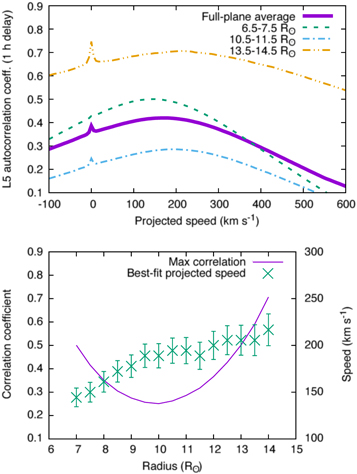
Figure 4. Shifted autocorrelation vs. radial lag across a 1 hr offset in the L5 data reveals the average wind flow speed. Top: raw correlations show a broad peak around an average projected wind speed at each altitude. The whole corona average speed is 170 km s−1, with significant variation across the corona. We attribute the minor spike at 0 km s−1 to residual, uncorrected flat-field effects in the COR2 detector, especially in the faint outer portions of the corona. Bottom: the wind speed gradually increases with altitude, reflecting the ongoing acceleration of the solar wind at high altitude. The peak correlation coefficient decreases at mid-altitudes and gradually increases again, possibly reflecting greater radial structure and intermittency in the outer corona.
Download figure:
Standard image High-resolution imageIn addition to determining a global average projected speed, we measured the average plane-of-sky projected speed in several 1 R⊙ wide bands, centered 0.5 R⊙ apart, throughout the field of view. The results are plotted in the bottom panel of Figure 4. Error bars in the lower panel are calculated using the width of the correlation peak in the smoothed plots in the top panel, folded into a posteriori estimates of rms error in the height of the correlation curve in each radius bin. There is an immediately obvious systematic shift (average acceleration) of the solar wind across this altitude range. Moreover, the correlation coefficient begins high (as might be expected from the strong signal at low altitudes) and drops with altitude, reaching a minimum at about 10 R⊙ before (surprisingly) rising again through the outer portion of the field of view. This intriguing result is discussed further in Section 4.2.
We used the measured projected wind speed to determine an approximate comoving frame in the image plane and to carry out time averaging in that comoving frame and minimize motion blur. To optimize the averaging for the outer portion of the field of view, where the S/N is the lowest, we used the high value of 220 km s−1.
The adopted projected wind speed of 220 km s−1 translates to 6.3 pixels per frame in the 800-pixel tall radialized L5 images. We replaced each frame with a Gaussian-weighted average of the nearby frames in this 220 km s−1 moving reference frame, using a 1 hr full-width Gaussian-weighting function enumerated over a 2.5 hr full width. Further, noting that the images themselves were blurred by motion during each exposure, we also smoothed vertically in each frame by convolution with a Gaussian kernel with a full width of 8 pixels, enumerated over a 24 pixel full width. The resulting frames, averaged across time in the moving frame of reference and also slightly smoothed radially, we called "L6." The L6 frames have no visually obvious "snow" or similar noise and reveal much more lateral structure than is present in the L5 frames.
We reconstituted the original brightness gradients by remultiplying each row of pixels in the L6 data by the corresponding measured standard deviation from the L4 data and adding back the measured mean brightness from the same images. From each frame, we then subtracted a pixelwise-minimum value, similar to the F coronal subtraction used to carry L1 to L2 data above. This resulted in a positive definite image sequence of feature-excess radiance: low-noise coronal images in photometric units, in polar coordinates, containing only transient bright structures. We called these data "L7." A sample frame at L6 and at L7 is in Figure 5. To present the data uniformly despite the reconstituted radial brightness gradient, the bottom panel of Figure 5 is scaled by the cube of the apparent radius from the Sun, following DeForest et al. (2016).
Figure 5. Same frame as in Figure 3, after radial smoothing and correction back to feature-excess normalized brightness, which reveals a "cleaned" corona. Top: "L6" frames lack the photon noise apparent near the top of the L5 frames. Bottom: "L7" frames contain true feature-excess brightness. This figure is also available as an animation. The animation starts at 2014 April 14 00:41:00.005 UT and ends at 2014 April 16 23:26:00.004 UT. Its duration is 56.5 s.
(An animation of this figure is available.)
Download figure:
Video Standard image High-resolution imageFinally, for a direct comparison to the original L2 data (Figure 2), we transformed the data back into focal plane coordinates to obtain "L8" images. Figure 6 compares a radially filtered version of the same L2 frame as in the prior figures, with the corresponding radially filtered L8 frame. The top two panels show the whole corona; the lower two show a close-up of the northwest quadrant. The additional smoothing improves the feature contrast and reveals features that are hinted at by the L2 data, at a cost of anisotropic smoothing/blurring of features moving at speeds greatly different from the modeled 220 km s−1.
Figure 6. Comparison between radial-filtered L2 data, scaled by the cube of the apparent radius (left two panels) and processed L8 data (right two panels), which reveals the effect of comoving-frame averaging. Top: full-corona view. Bottom: close-up of the northwest quadrant. This figure is also available as an animation. The animation spans the same time range as that of Figure 5.
(An animation of this figure is available.)
Download figure:
Video Standard image High-resolution image3. Analysis and Results
The processed COR2 data have very low noise compared to prior studies, and they therefore reveal considerably more and finer detail in the outer corona than has been apparent in prior analyses with COR2 or with SOHO/LASCO. We therefore present initial results of several types of analysis acting on the deep-field images, both to characterize the outer corona and to indicate directions of important future work that are now enabled.
3.1. Visual Analysis
The L7 and L8 images reveal a great deal of fine-scale structure across all position angles and radial distances, even by simple inspection (Figure 7 and its animation). The animation shows a plasma outflow that is radial, at least within the COR2 field of view; intermittent, so that small density fluctuations form an optical flow; and somewhat inhomogeneous. The occasional CMEs—we counted six during the 3 day campaign—propagate faster than this background flow, as expected. One of them, however, is slow enough to be indistinguishable from the background flow in individual snapshots and can only be detected by the coronal depletion in its wake. The slow CME extends between a position angle of 100°–170°, starts at about April 14 14:36 UT, and ends at April 16 ∼4:36 UT. At other locations, we detect the familiar blobs (e.g., PA 250°–270° between April 14 00:00 UT to April 15 03:00 UT) behind a CME that erupted the day before.
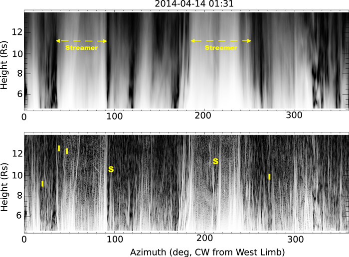
Figure 7. Top: an L7 snapshot (see also Figure 5) annotated with several features of interest. Bottom: the same image treated with the Sobel operator (see the text) to highlight brightness gradients (edges). The feature intensity in this image is proportional to the slope of the brightness gradient in the original image. The letters "I" and "S" mark examples of intermittent and smooth radial flow.
Download figure:
Standard image High-resolution imageThe L7 (and L8) time series also reveal a highly filamentary and intermittent fine-scale structure within the coronal streamers. Although there have been indications of such structure in previous studies (Thernisien & Howard 2006), the combination of the COR2 deep-exposure and high cadence observations with the background treatment described in Section 2 make it very clear (see Figure 8 and its animation). Each streamer comprises several filamentary striae of varying widths, spacing, and brightness. The analysis in the next section indicates that these features are well above the remaining noise floor. They may be either individual features or small-scale folds of the 3D plasma sheet that permeates the streamer. What is not so clear in the still images of Figure 6 is the ubiquitous variation of the emission along the individual striae, which gives a visual impression that they may be formed by a continuous train of intermittent structure rather than a smooth flow.
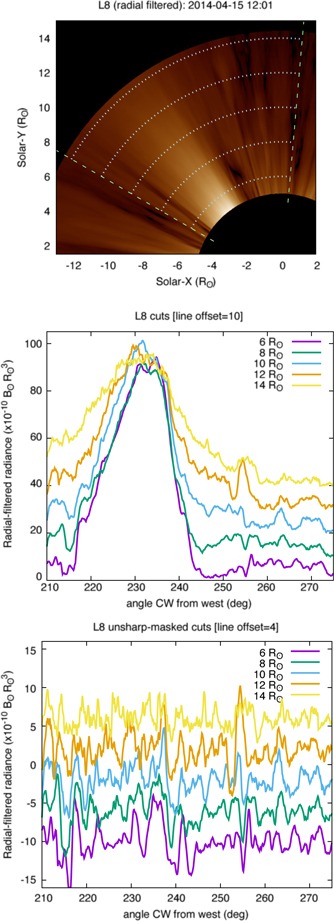
Figure 8. Detail image and plots from the north and northeast regions of the corona reveal persistent, fine radial structure. Top: detail image shows a wide streamer and a small polar coronal hole. Middle: plots of radial-filtered radiance at five altitudes show both large and small radial structures. Bottom: unsharp-masked plots reveal fine structure at all locations in the images.
Download figure:
Standard image High-resolution imageTo enhance these small-scale patterns, we further processed the L7 images with the Sobel edge-detector operator (e.g., Petrou & Petrou 2010), which yields the magnitude of the discrete gradient of the image at every point. The resulting image is shown in the bottom panel of Figure 7. Under edge detection, it is apparent that the two large streamers are not composed solely of filamentary structures, but also contain areas free of strong visual edges (e.g., angles 60°–70° and 190°–210°). Those areas become more prevalent above about 9 R☉ across most position angles (azimuths). Along a given radius, however, the Sobel algorithm detects multiple edges (displayed as short spikes in the image). These edges show that the brightness along that radius is particularly nonuniform.
The Sobel-enhanced time series (visible in Figure 7's animation) reveals that the strong intermittent features are flowing outward. Several regions containing these strong, intermittent features are labeled with the letter "I" (for "intermittent") in Figure 7. On the other hand, the streamer edges (labeled with the letter "S") appear quite smooth with a strong gradient in the azimuthal direction only. Since most streamer stalks likely mark folds of the plasma sheet (Howard & Koomen 1974), the apparent uniformity in these locations could be due to a longer line-of-sight integration that smooths out the intermittent structures. At least some of the intermittent outflowing features may be associated with evolution in the low corona; an inspection of images from the Solar Dynamics Observatory/Atmospheric Imaging Assembly around the time of the appearance of the blobs in position angles 250°–270° showed several quiet-Sun brightenings in those locations originating over bright points and somewhat more extended regions. We defer further analysis of these possible associations to a future study, focusing instead on analyses of the features themselves and their implications for the outer corona.
3.2. Universal Fine-scale Structure
A striking aspect of Figure 6 is the ultra fine radial structure of the outer corona, which contains both the familiar striae on 1°–2° scales in the position angle (e.g., Fisher & Guhathakurta 1995) described in Section 3.1, and also far finer striae, with the anisotropic appearance of grain in a rip-cut hardwood board. The large-amplitude portion of this structure is apparent in Figure 7, but the "woodgrain" appearance extends to yet smaller scales.
To characterize and interpret this structuring, we analyzed a single image in more detail. Figure 8 shows a region containing both a wide streamer and a coronal hole (identified by their morphology and corroborated using concurrent magnetic extrapolations from the GONG network) and plots radiance on constant-radius cuts through the region, as marked in the top panel. The woodgrain texture of the image is reflected in myriad small bumps in the plots. The bottom panel of Figure 8 shows the difference between each pixel's value and the Gaussian-weighted mean brightness of surrounding pixels at the same radius. The Gaussian-weighting function has a full width of 4° of azimuth, eliminating large bright features, such as the streamer itself (near 230° azimuth). The individual plot traces are offset vertically for comparison between them. The long radial striae of the corona are reflected in (some) features that are persistent across three or more of the plots in the bottom panel of Figure 8.
It is not immediately apparent, from examining the bottom plot in Figure 8, how much of the variation in the traces is significant and how much is random noise. To distinguish the coronal signal from noise, we analyzed the second-order structure function of the Figure 8 image, as described by DeForest et al. (2016).
The second-order structure function S2 of a 2D image  can be used to characterize image structure without reference to particular features in an image. It is just:
where the Δ variables are called "lags." Because the difference between nearby pixels is squared, S2 may be averaged or cut over one or more of its four dimensions to explore the structure of an image. The second-order structure function is developed in more detail by DeForest et al. (2016) and references therein.
Figure 9 shows vertical and horizontal cuts through the lag axes of S2 that correspond to the frame in Figure 8, from the L3 and L7 steps of analysis. Each panel of Figure 9 shows the average of S2 across the azimuth (x), with the radius (y) held constant, with either  for the vertical cuts or Δy = 0 for the horizontal cuts. The top panel shows cuts at 14 R⊙ and clearly shows the effects of noise on the images. At zero lag, S2 ≡ 0, because each pixel has the same value as itself. Adjacent pixels are affected by noise, and this is reflected in a flat, nonzero value of the L3 structure function cuts in the vicinity of zero lag. The horizontal and vertical cuts rise with different slopes far from zero lag, highlighting the familiar coronal anisotropy. The L7 horizontal and vertical cuts have lower values near the origin, approaching the identical zero point with zero slope, and there is no visible offset at this plotting scale. This reflects deep suppression of the noise by the L3-to-L7 processing described in Section 2.

Figure 9. Lag-axis cuts through the azimuthally averaged second-order structure function of the image shown in Figure 8, in polar coordinates, reveal gradual isotropization of the corona and also the noise characteristics of the L3 and L7 images.
Download figure:
Standard image High-resolution imageBy noting that the expected noise-free form of S2 has zero slope at zero lag, it is possible to estimate the noise level in the L3 and L7 data based on the value of S2 in the vicinity of the lag origin. If noise in adjacent pixels is truly uncorrelated, the S2 value at the first pixel with nonzero lag in each direction should reflect the noise level. Because the L3 data have had nontrivial resampling steps applied to them, it is possible that adjacent pixels are slightly correlated by the interpolation operation from L2. We used the average of the S2 values from (Δx = ±4,  ) and (Δx = 0, Δy = ±5) in L3 pixel coordinates. That distance is great enough to ensure an uncorrelated sampling at 6 R⊙ in the original image plane and is short enough (based on the shape of the curves in Figure 9) that S2 is dominated by noise there. The estimated noise level is (ΔS2/2)0.5, because the difference represents the uncorrelated sum of two samples of additive noise.
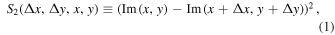
Figure 10 shows the noise level inferred from the notch depth. It varies monotonically from  to
to  , with a single jump near the outer vignetting minimum of the instrument. The vignetting minimum manifests as a faint ring of higher photon noise between 11 and 12 R⊙. It can also be seen as a residual error in the F corona estimation, forming bright rings in the L2 image in Figure 2.
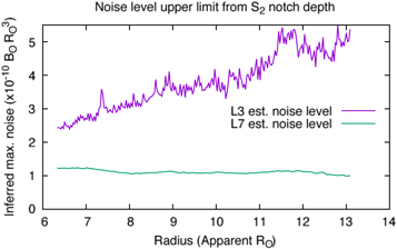
Figure 10. Azimuthally averaged L3 and L7 upper-limit noise levels vs. the radius in the region of interest from Figure 8. The upper limit is determined from the height of the zero-lag "notch" in the L3 structure function cuts and varies in an expected way across the field of view. The L7 cuts have no significant notch, and the curve is instead dominated by image structure rather than noise. An analysis of the fluctuations in the two curves reveals the L7 noise level.
Download figure:
Standard image High-resolution imageThe lower curve in Figure 10 is the noise level estimated by the same method from the L7 data. It is a factor of 2.5–5 lower than the noise level in the L3 data, at roughly  . However, this is a weak upper bound for the actual noise level; the height of the notch includes both image structural and image noise effects and therefore gives only an upper bound for the noise level. The shape of the notch in the L3 cut shows that the image structure is negligible compared to the noise. But there is no visible notch in the L7 cut; the height of the L7 S2 cut is dominated at 4 pixels (0
 4 azimuth) by the image structure itself.
Fortunately, there is a secondary approach to noise estimation. The pointwise L3 estimated noise level curve itself includes statistical fluctuations, which are a reflection of statistical sampling of the very noise being measured. We can use these fluctuations as an independent-from-the-mean measure of the noise level.
Between 9 R⊙ and 10 R⊙, the L3 curve in Figure 9 has a mean value of  . Removing the linear trend yields a standard deviation about the trendline of
  . Performing the same operation on the L7 curve yields a standard deviation about the trendline of
  . By this measure, the noise level in the L7 data is reduced by a factor of 14 compared to that of the L3 data. We infer that the processed data therefore have typical noise levels of the order of
  .
.
We conclude that the  fluctuations in the cuts in Figure 8 are real image structures some 10× stronger than the L7 noise floor.
Having demonstrated that the structures in the Figure 8 cuts are significant, we can estimate the density variation they represent if they are singular structures and not coincidences of multiple structures along the line of sight. A typical structure amplitude and width in the 14 R⊙ trace in the bottom panel are 4 × 10⁻¹⁰ B⊙  and 05, respectively; these correspond to 1.5 × 10⁻¹³ B⊙ and 0.12 r⊙, respectively.7
Surmising an out-of-plane aspect ratio close to unity, this amplitude and scale afford direct inversion to estimate each feature's density, using the small-Sun approximation and following Howard & DeForest (2012). If the feature lies within the Thomson plateau, then Howard & DeForest's Equation (6) reduces to:
and 05, respectively; these correspond to 1.5 × 10⁻¹³ B⊙ and 0.12 r⊙, respectively.7
Surmising an out-of-plane aspect ratio close to unity, this amplitude and scale afford direct inversion to estimate each feature's density, using the small-Sun approximation and following Howard & DeForest (2012). If the feature lies within the Thomson plateau, then Howard & DeForest's Equation (6) reduces to:

where ne,feat is the density of the feature under study, Bfeat is its radiance, sfeat is its estimated depth, and

contains the solar brightness, B⊙; the solar radius, r⊙; the Thomson scattering cross section, σt; the Sun-observer distance, Dobs; and the observing elongation angle, ε. Applying Equations (2) and (3), we arrive at  in these bright features, at an apparent distance of 14 R⊙.
By comparison, taking the typical solar-wind density and speed at 1 au to be 6 cm−3 and 400 km s−1, the typical background number density at 14 r⊙ with a local flow of 200 km s−1, from conservation of mass, is 3 × 103 cm−3, an order of magnitude lower than the computed feature density.
We infer that the fine-scale ("woodgrain") structure observed in the L7 and L8 images is real and not modified noise, and reflects highly inhomogeneous density structure in the outer corona, with fluctuations of the order of 10× the average density on scales below 02 of azimuth. This structure has not been visible in prior studies, primarily because it exists well below the noise floor of most coronagraph images.
The spatial fluctuations in Figure 8 reflect a broad spectrum of feature sizes. To quantify how their amplitude varies with size, Figure 11 shows the azimuthal spatial brightness spectrum, which closely follows a power law with  . The spectrum covers frequencies up to 3.5 deg−1, which correspond to features of 015 in width.
Figure 11. Azimuthal brightness spectrum along the 10 R⊙ cut in Figure 8 closely follows a f−1.5 power law, reflecting an f−1 dependence of density amplitude on a spatial scale.
Download figure:
Standard image High-resolution imageBy taking lateral feature size to an approximate line-of-sight feature size and assuming that the number of features N(f) along each line of sight is proportional to f—and that therefore their incoherent sum yields an f0.5 dependence—we can write the relationship between density, brightness amplitude A, and spatial frequency f as:

We conclude that the underlying density spectrum has power f−1 throughout the observable range of scales, down to the limit of our analysis at approximately 015 of azimuth. At 10 R⊙, that scale corresponds to features subtending just 27 arcsec (20 Mm) on the sky, or two COR2 detector pixels.
3.3. Ubiquitous Compact Features
In Section 3.1, we noted compact bright features that appear to be intermittent density fluctuations along certain radii. To highlight and characterize these features, we further enhanced the L8 data by unsharp masking in time; from each frame in the L8 time series, we subtracted a Gaussian-weighted average brightness of the surrounding interval of time centered on the relevant frame. The Gaussian-weighting function had a full width of 2 hr.
Figure 12 and its animation show the result of this unsharp masking and reveal that the small bright features ("blobs" and other features) are ubiquitous, even in regions identified as steady in Figure 7. In those regions, fluctuations are still apparent in the unsharp-masked image and animation, but they are too faint to register as well-detected edges using the Sobel transform directly on the L7/L8 data.
Figure 12. Temporally unsharp-masking L8 data reveals that propagating brightness fluctuations are present at all azimuths and times, with a wide range of brightnesses and lateral sizes. The animation of this figure matches the temporal characteristics of Figure 6.
(An animation of this figure is available.)
Download figure:
Video Standard image High-resolution imageThe features propagate with a variety of speeds but appear to form local tracers of the "typical" plane-of-sky projected wind speed; we make use of this property in measuring the wind speed in Section 3.4. Further, they appear to represent an extended family of features that includes the "Sheeley blobs" at the large/bright end of the size distribution. These bright features are analyzed further in Section 3.5.
The outward propagating blobs and other intermittent bright features show an anisotropy of structure; their smallest spatial scales are longer in the radial direction than the surrounding striae are in the azimuthal direction. That radial length can be attributed directly to motion blur, both on the detector of COR2 and (in most features) in the postprocessing. Recall that the L7 and L8 frames were created by averaging in the radial direction (making use of the existing motion blur) and in time, in a moving frame of reference. The moving frame used a single outflow speed for the entire corona; but individual features in Figure 12's animation can clearly be seen to be moving at different speeds. This mismatch exacerbates any motion blur already present.
3.4. Wind-speed Measurement
In the course of preparing the images (Section 2), we measured the average apparent feature speed versus plane-of-sky projected altitude, using a peak in the offset autocorrelation function (Figure 4). In light of Figure 12, the reason for the success of this method becomes apparent. The offset autocorrelation function was detecting propagation of the ubiquitous intermittent brightenings seen in Figure 12.
Here, we compare that measurement to a different indicator of solar-wind speed: average coronal brightness versus altitude. Under steady flow conditions, simple conservation of mass and the inverse square law dictate that coronal radiance should fall as the cube of distance from the Sun. Increased flow speed must, on average across the whole corona, be matched with a proportional decrease in density. Since Thomson scattering is a linear process, this corresponds to a proportional decrease in brightness. We used the radial falloff in the average brightness of the L5 images, across the entire data set, to corroborate the apparent acceleration visible in Figure 4.
The correlation-derived solar-wind speed is a projected speed in the focal plane of the instrument. However, each pixel represents a long line-of-sight integral through the corona, and "typical" K-coronal features are displaced from the focal plane rather than in it. This is discussed in detail by DeForest et al. (2016) and results in a "most typical" feature distance that is 1.09 times the apparent (projected) distance from the Sun of each line of sight. We infer that the actual typical wind speed in 3D is greater than the plane-of-sky projected speeds in Figure 4, by the same factor of 1.09.
Figure 13 compares the measured radiance falloff with radius, to the speed profile inferred via correlation tracking and corrected for geometry. Formal error bars on the coronal brightness are negligible because the value is an average across time and space in the entire data set; each brightness value is the average of approximately 8000–48,000 independent measurements. Systematic errors may exist and are not accounted for by this simple analysis.
Figure 13. Solar wind undergoes extended acceleration in the outer solar corona. The result is corroborated by two separate measurement techniques: autocorrelation as in Figure 4, and anomalous radial falloff of the coronal radiance. See the text for a discussion of uncertainty and error.
Download figure:
Standard image High-resolution imageThe most likely source of systematic error in the radiance measurement arises from the fact that the radiance being measured is feature-excess radiance, rather than the true full integrated radiance of the corona along each line of sight. Variation in the intermittency or structuring of the corona may affect the relationship between the measured feature-excess radiance and the true radiance of the corona. This could be overcome by analyzing polarized brightness (pB) images of the corona from COR2, which permit a direct measurement of the actual coronal brightness by the direct subtraction of the nearly unpolarized F corona. We defer that more in-depth analysis to future work.
The two axes in Figure 13 are scaled linearly, and the two curves would therefore overlay one another perfectly if solar-wind acceleration were the only effect shifting the overall radiance. Agreement to within 10% in slope (as is seen in Figure 13) is reasonable corroboration that the two effects are both measuring solar-wind acceleration, but are subject to the caveat in the previous paragraph.
We conclude that the solar wind, averaged over the entire corona, undergoes continuous acceleration throughout the altitude range imaged by STEREO/COR2 under "typical" solar-maximum conditions, with speeds as low as 200 km s−1 even at 10 R⊙ or higher.
Solar-wind speeds in the corona have been measured by the method of radio scintillation (e.g., Armstrong & Woo 1981), with a factor-of-four variation in speeds in the same altitude range. Armstrong & Woo, in particular, found speeds in the range 70–325 km s−1. Our results are skewed toward the lower range but are not inconsistent. In particular, the peaks in Figure 4 are broad in part because of motion blur and in part because of the range of observed propagation speeds, and the breadth encompasses the full range of radio-observed speeds. Further, both the visible and radio measurements are weighted line-of-sight averages, and the weighting functions almost certainly differ, so that if (as observed) a range of speeds is present, different measurements may highlight different portions of that range.
Obvious next steps include azimuthal analysis to search for high-shear regions that could give rise to hydrodynamic instabilities (e.g., DeForest et al. 2016); time-domain analyses to determine variability of wind acceleration and flow; more thorough characterization of the (kr, ω) Fourier plane to identify possible wave modes and interactions; and brightness/speed studies enabled by discrete tracking of individual features ("blobs") and other inhomogeneities, as discussed below.
3.5. Analysis of Blobs
To further characterize outflow and understand the transient features—hereafter called "blobs," because the large ones associated with helmet streamers appear to be "Sheeley blobs" (Sheeley et al. 1999)—we analyze the trajectories and densities of several representative examples from the bright end of the distribution apparent in Figure 12. We focus on position angles 250°–251° where there was considerable bright blob activity on 2014 April 14. First, we investigate their kinematics by constructing time-distance maps (so called "J-maps," Sheeley et al. 1999). We averaged radiance over a 1°-wide angular sector (PA 250°–251°) in each "L7" image over one full day and plotted brightness versus time and height in that sector. The resulting J-map (Figure 14) shows numerous diagonal stripes, indicating feature motions.
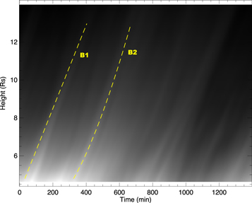
Figure 14. Height–time map produced by averaging PA 250-251 during 2014 April 14. Blob ejections are shown as inclined stripes where the slope depends on the blob speed. We analyzed the kinematics and densities of two blobs, labeled "B1" and "B2" and their traces marked by the dotted lines.
Download figure:
Standard image High-resolution imageThe brightest and sharpest traces in Figure 14 correspond to Sheeley blobs. Two of those blobs are labeled "B1" and "B2," and their traces are marked with dotted lines. The slope and shape of each trace are directly related to the speed profile of the feature; faster features have steeper slopes, and accelerating features are characterized by concave upward slopes. We extracted the height–time and brightness profiles of the two blobs by manual tracing. We fitted the height–time profiles with parabolas to derive their kinematics (Table 1); we report the plane-of-sky apparent speed only. Both blobs exhibit gradual acceleration. The blob radial speeds, 300–400 km s−1 at 13 RSun, are consistent with past measurements (e.g., Sheeley et al. 1997), suggesting that they propagate within the general solar-wind flow—although their motion is faster than the overall speeds found in Section 3.4 for the ensemble of moving features as a whole. Sheeley et al. (1997) measured blobs that occurred at a range of speeds for a given height, and that range encompasses the speeds found in Section 3.4. There are also yet faster outflows in Figure 14, as suggested by intersecting traces. However, most of the large and bright features yield slopes that are quite similar to each other and to the B1 and B2 slopes.
Table 1. Kinematics of Blobs
| Height Range | Speed Range | Acceleration | |
|---|---|---|---|
| (RSun) | (km s−1) | (m s−2) | |
| B1 | 4.9–13.2 | 199–299 | 2.2 |
| B2 | 4.8–13.1 | 200–390 | 5.7 |
Download table as: ASCIITypeset image
Since the L7 images are calibrated in excess mean solar brightness, it is relatively straightforward to estimate the excess density8 of the blobs as a function of height. We apply the standard formulas for calculating the number of electrons (per cm2) from the excess brightness (e.g., Vourlidas et al. 2010; Howard & DeForest 2012, and references therein). To estimate the volumetric excess electron density, we assume that the blob depth equals its width in the L7 images, which is about 1° for B1 and B2. This is a commonly used assumption for small compact features. A constant angular depth (and width) implies that the blobs expand self-similarly. Since the actual depth is unknown, we consider only the systematic errors in the density estimation. The systematic errors are discussed in detail by Vourlidas et al. (2010) and shown in their Table 1. The dominant errors are (1) the background subtraction (estimated at 4%), and (2) the compositional uncertainty of 6% because the plasma composition on these small blobs may vary significantly from the average composition over the much wider CME areas. Since the errors are independent, the combined error is estimated to be 7.2%. Photometric uncertainty in the L8 data is negligible by comparison.
The resulting density profiles for B1 (solid) and B2 (dashed), including the 7.2% error bars, are shown in Figure 15. The excess densities drop from ∼5.8 × 10⁴ to 7.2 × 10³ or roughly a factor of 8 between 4.8 and 12 RSun. This is slower than expected for adiabatic expansion (∝r−3 or factor of 17 for the heights considered here). We infer that, under the assumption above, these blobs are either constrained (by internal magnetic fields or the ambient pressure) or pile-up upstream material as they expand.
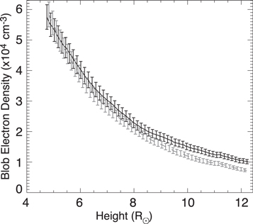
Figure 15. Electron volume density evolution in blobs "B1" (solid line) and "B2" (dashed line), which were traced in Figure 14. We assume a line-of-sight depth equivalent to 1° in azimuth (0.08–0.2 R⊙ across the altitude range) to derive the volumetric density estimates. As the actual depth is unknown, we consider only potential systematic errors, which amount to 7% (see the text for details).
Download figure:
Standard image High-resolution imageNote that the densities inferred for these bright blobs are about 10× smaller than the densities inferred for bright thin striae in Section 3.2. This is because these brightest blobs have comparable radiances but larger widths (hence larger inferred line-of-sight depths) to the features analyzed there.
Next, we quantify the timescale of a series of solar-wind blobs seen in the corona. Position angle 240° is another area that exhibited density blobs that appeared to be continually released from the Sun quasi-periodically, with a timescale of roughly 20 minutes. Quasi-periodic blobs occurring at such short timescales have never before been observed close to the Sun, though in situ observations at 1 au have suggested their existence (e.g., Viall et al. 2009; Kepko et al. 2016). The deep exposures of this special observation run, coupled with the rapid time cadence, allow us to probe this shorter timescale for the first time. Importantly, this activity is visible at each of the levels of data processing (i.e., L2–L8), confirming the physical nature of the blobs, though they are most striking to the eye in the L8 animations.
We performed a spectral analysis on this region to quantify whether or not the density structures are released quasi-periodically, i.e., with a characteristic timescale. We summed the L5 image data over a "virtual slit" that is 10 pixels wide (equal to one degree of position angle, from 239° to 240°) by one pixel in the radial direction and computed the time series of the summed pixel value as a function of time. The pixel slit is located at a height of 4.9 R☉. We plot the intensity time series in Figure 16 over an interval of 23.5 hr beginning at 2014 April 14 00:41 UT. The brightness variation produces a signal analogous to the density that an in situ spacecraft would measure at the location of the blobs, as the solar wind advects past.

Figure 16. Intensity time series showing the passage of density structures using the L5 data through a slit of pixels between 239° and 240° at a height of 4.9 R☉ during 2014 April 14.
Download figure:
Standard image High-resolution imageWe found the L5 data to be the best to work with for this purpose, as they have the background subtraction and star field removal but not the heavy smoothing of the L7 and L8 data. The smoothing step would reduce the effective time resolution for this measurement, due to the increased motion blur from the mismatch between the whole corona average speed and the local speed of the particular blobs of interest.
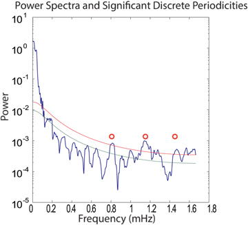
We performed a spectral analysis on this intensity time series following the multitaper method of Mann & Lees (1996). This method has been applied both to time series of solar-wind density data and white light imaging data (Viall et al. 2008, 2010; Viall & Vourlidas 2015). We plotted the power spectra and results of the significance tests in Figure 17. The power spectrum is shown in blue, and we plot the background approximation, which we take to be a first order autoregressive function, in green. Physical systems (including the solar wind) typically have time series spectra that exhibit higher power at lower frequencies and lower power at higher frequencies (sometimes called a red spectrum). The autoregressive function is approximately a power law and physically it represents a system that has memory (Ghil et al. 2002).
Figure 17. Spectral estimate computed with the multitaper method (dark blue). We show the background estimate is shown in green, and the 95% confidence threshold in red. Circles indicate periodicities that had significant power and also passed a harmonic F-test.
Download figure:
Standard image High-resolution image
In red, we show the 95% significance threshold for a narrowband enhancement of power relative to the background spectra. We perform the Harmonic F-test (Thomson 1982) in conjunction with the plot. The Harmonic F-test is a test of the phase coherence of a periodicity and is independent of the background in the spectral power. The red circles indicate periodicities that pass both the narrowband amplitude test and the Harmonic F-test at the 95% threshold simultaneously. The 20 minute periodicity (0.8 mHz) we identified by eye passes the combined spectral test. Two other periodicities at higher frequencies are also present, but are detected at a weaker level in the F-test and may or may not be physical.
Viall et al. (2010) and Viall & Vourlidas (2015) showed that the large-scale, hours-long trains of Sheeley blobs are composed of embedded, smaller-scale structures. Sanchez-Diaz et al. (2017b) expanded on these earlier studies and confirmed that large-scale blobs are composed of smaller-scale blobs. The smaller-scale structures are not randomly injected into the solar wind, but are injected quasi-periodically, with characteristic timescales of the order of 90 minutes. Viall & Vourlidas (2015) were limited by the 30 minute cadence of the COR2 data for the data set that they analyzed and could not determine whether quasi-periodic density structures occurred at even smaller scales. Here, we have shown that quasi-periodic density structures are also injected into the solar wind on timescales that are a factor of four smaller than those found by Viall & Vourlidas (2015) and Sanchez-Diaz et al. (2017a).
The obvious next steps in characterizing blob and solar-wind outflow include an automated analysis of the newly visible fainter end of the blob size and brightness distribution; association with lower coronal features to identify the origin of the blobs; 3D tracking using polarimetry; and deep-field tracking of the blobs into the young solar wind outside the corona to determine their effect on solar-wind flow and turbulence. A more thorough spectral analysis is needed, both in this data set and across the solar cycle, to determine potential mechanisms and the relationship between the newly detected higher-frequency blob release and the solar wind as a whole.
4. Discussion
The noise level and spatial resolution are intimately related. By reducing the background noise level by a factor on the order of 30 compared to typical analyses, we have revealed that the outer corona is far more highly variable and structured than is acknowledged by most work to date, including observations, numerical modeling, and theory. The preliminary results cataloged in Section 3 are individually surprising, but together form a coherent picture of an outer corona that is both very highly structured in space and intrinsically dynamic. Those dynamics extend beyond the simple wind acceleration and large-scale structures that have been observed, with steadily increasing resolution and fields of view, since the invention of the coronagraph.
This insight into the structure and nature of the outer corona has profound implications for several aspects of heliophysics, which we discuss in the following subsections.
4.1. The Spatially Structured Outer Corona
We observed spatial inhomogeneities in brightness that extend down to the smallest optically resolved scales of the COR2 instrument, apparently reflecting an intrinsic f−1 spectrum of density across magnetic field lines in the corona itself. This observation is relevant to the understanding of the connection between the dynamic "magnetic carpet" (e.g., Simon et al. 1995) and the outflowing solar wind, of the ubiquity of reconnection throughout the corona and solar wind (e.g., Tenerani et al. 2016), of the origins of solar-wind turbulence (e.g., Matthaeus et al. 1991; Cranmer et al. 2007; Matthaeus & Velli 2011), and of the nature of the Alfvén surface that divides the corona and heliosphere (e.g., Schwadron et al. 2010).
In principle, it is not surprising that the solar corona, where the magnetic field pressure dominates over the plasma pressure by up to two orders of magnitude, is structured by extremely fine-scale density structures that, at least approximately, trace the magnetic field. The coronal plasma originates in the complexly structured chromosphere, so transverse striations in density to the scale of photospheric or chromospheric structures, well below the supergranular scale, are to be expected. In fact, these types of directly connected magnetic domain structures are routinely observed near the surface of the Sun in the EUV. Further, the fine-scale magnetic domains and corresponding density structures are regularly observed in Thomson scattered light at solar altitudes of up to ∼3 R⊙ during total solar eclipses (e.g., Habbal et al. 2014, and references therein). The present observation demonstrates definitively that similar very fine striations, apparently shaped by the magnetic field, extend far into the outer corona, where the outflowing plasma transitions to become solar wind.
While the observation of very fine structure in the outer corona may "in principle" not be surprising, it is nevertheless "in practice" quite surprising. We have found that, just as the coronal loops seen in EUV (Tousey et al. 1977) essentially all contain unresolved image-plane structure down to the smallest observable scales (e.g., DeForest 2007; Kobayashi et al. 2014), so too do outer-coronal structures, such as streamers, pseudostreamers, plumes, rays, and related density structures ("striae").
We observed a continuous azimuthal spectrum of radially aligned density structures down to scales of approximately 20 Mm at 10 R⊙. With direct radial expansion, such structures would correspond to 2 Mm (∼2–3 granule) magnetic domains at the surface of the Sun. However, expansion of open regions through the lower corona is superradial. The linear expansion coefficient of bright structures between the bottom of the corona and 10 R⊙ is at least six in coronal holes (DeForest et al. 1997) and can grow much higher in the closed corona (e.g., Büchner 2006). This implies source structures in the chromosphere no larger than 300 km, or under half a granule, in scale. If in fact these smallest observable outer-coronal structures are directly connected to individual granules, changes on the granulation timescale ought to be directly observable; contrariwise, if chromospheric and coronal effects dominate the connectivity, the granulation timescale should not be particularly special.
A more quantitative analysis, via a structure function analysis of the brightness distribution, has revealed the ubiquity of large-amplitude, fine-scale density contrasts, with a spatial distribution following an f−1 spectrum down to the optical resolution scale of COR2. f−1 spectra, also called "pink" or "flicker-noise" distributions, are well known to arise in scale-free dynamic phenomena (such as sand-pile avalanches) and are observed at very low frequencies in the magnetic fluctuations in the solar wind (see, e.g., Bruno & Carbone 2005, and references therein). Lower down in the solar corona, temporal Lyα intensity fluctuations observed by UVCS have been interpreted as density fluctuations distributed according to an f−2 Brownian noise, from periods of a few hours to periods of a few days (Telloni et al. 2009). At higher frequencies, an f−1 window is also observed in time (Bemporad et al. 2008) and is distinct from the spatial spectrum reported here. On the other hand, the dynamical phenomena leading up to such a spectrum, namely reconnection and plasmoid merging (Matthaeus et al. 1991), which has been invoked for the time-domain spectrum, might also reasonably explain the spatial distribution observed.
Identifying whether the observed f−1 spectrum continues to smaller scales is of great interest because it provides clues to the origin of the observed woodgrain structure; if there turns out to be a spectral break at or near the scaled granulation size, it would imply that the outer-coronal woodgrain is a direct manifestation of the churning magnetic carpet at the photosphere; contrariwise, if there is not, it would lend strength to the idea that intrinsic dynamics of the corona itself give rise to these observed fine scales (e.g., Verdini et al. 2012).
Turning from the origin of the woodgrain to its implications for the state of the outer corona, we note that the inferred electron density variations are quite large, as are the variations in the observed speed across the population of blobs and smaller blob-like inhomogeneities (discussed below). This implies that the solar wind passing through the outer corona is far from homogenized; individual magnetic flux systems may carry different, nearly uncoupled streams of solar wind even as far out as 10–15 R⊙, providing a myriad of possibilities for hydrodynamic or MHD instabilities, including reconnection modes, as described by Matthaeus et al. (1991), to develop and drive local energy release in the outer corona. As a side note, reconnection inside coronal holes in the outer reaches of the corona has been recently invoked by Tenerani et al. (2016) as an explanation for inbound features seen in this altitude range. Our observation of strong inhomogeneity supports that work by showing that suitable conditions exist for small-scale reconnection to occur.
As a touchstone scale, we observed that, at 10 R⊙, many structures subtending ∼05 of azimuth (∼60 Mm across) appear to be 10× more dense than the average density of the solar wind at that altitude. Scaling with the inferred f−1 power law, the smallest observed structures vary by approximately 2–3× the average solar-wind density. This implies not only a strongly inhomogeneous wind but also a strongly inhomogeneous wave speed. In particular, the Alfvén speed, which varies as ρ−0.5, might be expected to shift by 40%–50% on 20 Mm scales and by a factor of 3 or more on 60 Mm scales. This inhomogeneity strongly affects the nature of the Alfvén surface (Verdini & Velli 2007; Schwadron et al. 2010; DeForest et al. 2014; Cohen 2015), also called the "heliobase," "Alfvén radius," or "Alfvén critical point," which marks the causal boundary between the corona and solar wind.
In the presence of large, fine-scale inhomogeneities in both the Alfvén speed and the wind speed, the critical transition from sub-Alfvénic to super-Alfvénic flow does not happen at a well-defined, smoothly varying radius—or, indeed, at any particular radius at all. Specifically, in the presence of large variations in wave speed, long-wavelength Alfvén and/or fast-mode waves must propagate at the spatially averaged wave speed in their vicinity, while shorter-wavelength waves may propagate inward through smaller loci where the wave speed is high, even though long-wavelength waves are advected outward by what, to them, is a super-Alfvénic flow. This adds further richness and nuance to the already very complicated physics of MHD wave-plasma interaction in the critical outermost zone of the corona. However the microphysics and other nuances play out, it is clear that there can be no smooth, well-defined, clean Alfvén-surface boundary. Rather, one should speak of an "Alfvén zone" in which each packet of solar-wind plasma separates gradually from the corona rather than passing through a clean "MHD event horizon." Further experimental understanding of this zone, and exploration of its consequences, will require a combination of still-deeper exposures of the outer corona, possibly from a coronagraph mission specifically designed for this purpose, and in situ measurement of the actual wave and flow speeds in the outer corona, from the upcoming Parker Solar Probe mission.
4.2. The Temporally Structured Outer Corona
In addition to surprising levels of spatial variation, we found ubiquitous small-scale "blobs," which appear to form a spectrum of sizes and densities. The largest of these blobs appear to be the long-observed "Sheeley blobs," which are revealed as representing one end of a distribution of small outflowing structures; but, as with the quasi-stationary striae, the distribution of features extends to quite small features. These features yield insight into the intermittent origin and flow of the slow solar wind and reveal a puzzling aspect of coronal evolution near 10 R⊙.
The dense striae discussed in Section 4.1 are important because, in general, coronal density traces magnetic field topology: both trivially because closed loops are denser and visible in emission EUV and X-rays, and also less trivially by outlining specific regions of topological interest. These regions include streamer stalks at forming current sheets, spine-fan structures of pseudostreamers, or, more generally, regions with high "squashing factors," which generally neighbor x-lines marking boundaries between multiple magnetic domains (e.g., Titov 2007). Not coincidentally, these are regions where small perturbations can lead to loss of plasma confinement—for example, via interchange reconnection—and therefore plasma blobs of enhanced density may be released. More generally, any perturbation propagating in such regions will end up focusing or steepening in the neighborhood of such quasi-separatrix layers, enhancing dynamically intermittent behavior there.
The first quantitative result in the time domain stems from an analysis of the shifted autocorrelation versus the radial lag of the L5 data. The peaks in the 1 hr offset autocorrelation coefficient reveals an estimate for the average wind flow speed across azimuth at the given height. We showed that the result, which reveals a consistent, slow acceleration from about 140 km s−1 at 7 R⊙ up to above 200 km s−1 at 14 R⊙, is consistent with an independent estimate coming from the analysis of the anomalous radial falloff of the coronal radiance (Figure 12). This comparison both lends confidence in the correlation measurement, and also strengthens the idea that the intermittent density structures (which are used for the correlation speed estimate) follow the acceleration profile of the wind itself; if there are separate intermittent and smooth components to the solar wind, they at least accelerate with approximately the same profile.
The unsharp-masked image sequence (Figure 12 and its animation) highlights the importance of a more detailed analysis of this flow speed. Features of all azimuthal sizes can readily be seen to be propagating at many different speeds in the image plane, and it is no trick to identify high apparent velocity shears. For example, features at adjacent position angles, separated by as little as 02, are readily seen to pass one another while propagating. While, in this introductory work, we do not analyze this shear field in detail, it seems clear that, just as adjacent striae can have quite different masses (as discussed in Section 4.1), they can (and typically do) also have quite different flow speeds. This strongly spatially structured flow, which is highlighted by the different outflow speeds of features on adjacent striae, is important for three major reasons.
First, the strong shear field of the observed differentiated flow is a potential energy source for the turbulent cascade that is thought to isotropize solar-wind structure (e.g., DeForest et al. 2016) and, ultimately, provide heat to the solar wind throughout the inner solar system (e.g., Leamon et al. 1998). One may surmise that this process involves generation, propagation, and mutual interaction of Alfvén waves from multiple instabilities and/or reconnection associated with the shear flow and density inhomogeneities.
Second, the intrinsic differences between flow at different position angles, coupled with the very fine woodgrain structure, support a magnetic picture of the young solar wind as a "mat" of tangled magnetic carpet flux structures, each carrying relatively independent streams into the heliosphere, rather than as a smooth flow through the outer corona (e.g., Crooker et al. 1996; Borovsky 2008).
Third, the broad range of transverse scales observed is an important clue to the nature of the solar-wind source and average solar-wind acceleration throughout the corona. The fact that features exist from the smallest observable scales to a few degrees of azimuth strongly suggests that the individual features are not mere pistons piling up material along individual magnetic carpet associated field lines. Like the flocculae that form in the young solar wind, these coronal blobs require collective motion across what otherwise appears to be different magnetic domains. This could be a manifestation of finite-size wave trains or (perhaps more plausibly) an indication that they are plasmoids that have been released individually and therefore have their own physical integrity via the tension force (Sheeley et al. 1999). With the additional smaller density blobs identified in this new data set, the blobs collectively might form a significant fraction of the solar wind, which is consistent with the observation of Viall et al. (2008) that periodic blobs with scales of 5–30 minutes comprised 80% of the in situ slow solar wind during a solar-maximum observation. The visibly variable component of the wind, as observed in Figure 12, sums to approximately 10% of the overall measured coronal brightness ("K") at each radius. Line-of-sight superposition effects ensure that this proportion is a deeply underestimated lower bound, implying that the spectrum of blobs does account for a large fraction of the visible solar wind. Determining that fraction is a subject for future work.
As presented in Section 4, the shifted autocorrelation function of the data contains a puzzling anomaly. The maximum (peak) lagged correlation coefficient, in particular, varies non-monotonically with altitude. The height of this peak initially decreases with height, reaching a minimum at about 10 R⊙ before rising again through the outer portion of the field of view. This is puzzling in part because, as we demonstrated in Section 3.2, photometric noise does not contribute significantly to the imaged features (and hence to evolution of the correlation coefficient). Some effect intrinsic to the corona is responsible.
We have come up with three possible hypotheses that might explain such behavior; a first, more obvious physical interpretation would attribute the decrease and increase of correlation to distinct sources of the density structures expanding into the wind. A first source arises in the low corona, and the second source arises somewhere in the neighborhood of the minimal correlation. In such a scenario, the correlation would first drop due to the mixing and rarefaction of the plasma blobs and then rise again once the enhancement from a second, higher source becomes dominant above a certain height. One would also expect then that the correlation should decrease again if one were able to follow structures further outward beyond the window used here with a sufficient S/N. It is more than reasonable to imagine a corona that contributes blobs of plasma to the wind starting from different heights, given the plausible height distribution of helmet streamer y-points and pseudostreamer fan-spines as well as the recent observation (DeForest et al. 2016) of the formation of turbulent "flocculae" at still higher altitudes.
A second possibility, which requires further in-depth study, might have to do with the loss of corotation of the expanding solar wind plasma. In this scenario, the radial region around the location of the minimum correlation would correspond, essentially, to an average over the latitude of the radial location where the solar wind becomes super-Alfvénic, i.e., where the solar coronal magnetic field no longer provides sufficient lateral (longitudinal) stresses to impose on the expanding plasma of a solid body rotation with the corona. Up until this height, the plasma longitudinal (rotational) velocity should increase in proportion to the radius, thus increasing the line-of-sight mixing effect of plasma streaming from the corona and appearing on the limb. Above the Alfvénic region, on the other hand, the azimuthal rotational velocity would decrease, essentially as R−1, leading to a smaller and smaller contribution of plasma from other longitudes to the measurement in the plane-of-sky. This might then lead to an increase of correlation with height above the region of corotation loss.
A third, more facile possibility that still needs to be eliminated is some sort of "kinematic" effect of the correlation itself. Because the Piersons correlation coefficient includes both steady effects from the coronal striae and also more sharply peaked effects from intermittent structure in the corona, interplay between the two classes of effects could cause nonintuitive variation in the peak correlation coefficient, even in the absence of a specific local physical process. In particular, radial variations in the relative strength of the steady and nonsteady components of the brightness, particularly in concert with the vignetting function of the instrument, could, in principle, mimic the anomalous signal shown. This idea forms a working "null hypothesis" and needs to be considered along with physical explanations in a more in-depth study to identify the cause of the observed radial dip in the time-lagged peak autocorrelation function.
Turning to more time-domain results, we have shown that at least some smaller-scale structures are not randomly injected into the corona, but are created with enhanced periodicities at timescales around 20, 40, and 60 minutes, which is smaller than the characteristic timescales of 90 minutes (2 × 10⁻⁴ Hz) found by Viall & Vourlidas (2015). Such periodicities may be due to local timescales interacting with magnetic reconnection (Kepko et al. 2016; Sanchez-Diaz et al. 2017a), though many plausible origins exist. These include wave propagation and resonance on magnetic field structures, such as helmet streamers, a cyclic breathing of the confined corona with pressure oscillations arising from the coronal heating process, or possibly also oscillations related to the global coronal structure itself. An example of such global structural oscillations is the coronal acoustic cutoff frequency that Pylaev et al. (2017) recently invoked to understand type-IV radio bursts and peaks at periodicities close to the 90 minutes of Viall & Vourlidas (2015).
So far in this discussion, a picture has developed of a far more complex, and causally disconnected, solar wind than is suggested by smooth flow models or hybrid models that treat a steady flow with a stochastic perturbation. In counterpoint to this picture, the observed similarity in Figure 13 between the acceleration profiles derived from intermittent structures and from photometry of the corona as a whole points toward a picture of the "background" wind arising via a blending of all of the subresolution emitted plasma structures or at least from momentum transfer between those structures. These two views are not necessarily inconsistent, but the full picture is clearly more nuanced than an either/or choice between a fully disconnected and stochastic solar wind and a smooth wind that is interrupted by sparse local structures (blobs) propagating through it.
5. Conclusions
We have produced the lowest-noise image sequence to date of the outer solar corona, using data from a special COR2 deep-field campaign and postprocessing to reduce noise further. The data were collected at solar maximum, so that it was not possible to fully and definitively separate coronal holes from "ordinary" slow solar wind. We have found that (a) essentially all coronagraphic images to date have had spatial resolution limited by intrinsic noise, leading to an erroneous impression that the outer corona is smooth; and (b) the outer corona is strongly structured in both space and time.
In particular, we have found that the brightest features in the outer corona, including streamers, pseudostreamers, and other striae, appear to be composed of smaller bright features all the way down to the optical resolution limit of COR2. This echoes similar findings in the lower corona from the Transition Region and Coronal Explorer (Handy et al. 1999) and the High Resolution Coronal Imager rocket (Kobayashi et al. 2014), which revealed that "coronal loops" seen with earlier instruments (Tousey et al. 1977; Walker et al. 1988; Delaboudinière et al. 1995) are apparently composed of far smaller strands. In the case of the outer corona, these individual dense strands are small enough that they could, in principle, correspond to individual granules or individual intergranular flux concentrations; there are also other potential explanations for the strands, including reconnection in the corona that gives rise to dense, semiconfined plasma in particular field lines.
The fine-scale structure we observe is sufficiently variable in density to complicate our understanding of the transition from the corona to the young solar wind; the critical Alfvén surface must at best be quite complicated with essentially fractal structure. Due to the expected interplay between wavelength and the effective Alfvén speed, it is better to think of this transition as a gradually disconnecting "Alfvén zone" in which inbound information flow pinches off gradually, rather than as a single well-defined surface akin to an event horizon.
Further, the spatial variability provides a potential energy storage mechanism to drive the observed turbulent cascade that is known to process, mix, and heat the solar wind on timescales of days.
In addition to the fundamental structural result, we find that the outer corona is highly nonstationary, with radially compact structures on multiple size scales. These structures account for 10% of the line-of-sight projected brightness of the entire corona during the observation, reflecting a higher percentage of the total density that is entrained in these fluctuations (most of which are almost certainly "washed out" by the necessary line-of-sight integral). The radially compact structures ("blobs") have a mix of scales and travel at widely varying speeds, though the overall trends are toward faster motion for brighter, larger blobs and for late-phase acceleration of a slow-moving solar wind—at least in the observed (maximum) phase of the solar cycle.
At least some of the blobs are produced quasi-periodically, pointing to semi-resonant release processes, such as reconnection instabilities involving resonance of dense structures, as well as to a speculated stochastic release from the direct evolution of the solar magnetic carpet. The blobs have a range of sizes, and most are larger than the finest-scale radial striae, indicating either a collective (wave) motion or plasmoid magnetic structure that imposes physical integrity through the magnetic tension force.
The compact structures, as an ensemble, produce an optical flow signal that can be used to extract solar-wind speed via shifted correlation between lagged images or via other related techniques. The lagged correlation signal behaves anomalously, pointing to as-yet unresolved physics in the vicinity of 10 R⊙ from the Sun. We have generated some hypotheses to explain this mysterious correlation dip and recovery, but further work is required.
Based on these preliminary results, we have identified many additional studies that require further, and more finely focused, effort to quantify and understand the rich set of phenomena revealed by the low-noise images. Some of these studies may be accomplished by further analyzing the present data set or additional similar sets to be collected by STEREO/COR2. Most of these studies require better instrumentation, such as a low-noise coronagraph optimized to study this transition to the young solar wind and/or a low-noise polarizing imager to extract additional 3D information via the physics of Thomson scattering.
We are prepared, based on our measurements, to make some predictions for the conditions the upcoming Parker Solar Probe mission will encounter in this part of the outer corona. We predict that the spacecraft will encounter strong, sharp variations in plasma density, by as much as an order of magnitude on timescales of 10 minutes or less. The correlation length of the plasma is expected to be under 50 Mm along the line of flight near in-corona perihelion passes.
In conclusion, the application of low-noise imaging has revealed a different, and far more complicated, outer corona than has been visible before. The outer corona is revealed to be at least as complex as the inner corona, with inhomogeneities, strong shears, and abundant and strong density fluctuations in both time and space. We have shown that these density structures can be tracked throughout the STEREO/COR2 field of view well below the sensitivity limits of prior measurements. This technique has already yielded abundant new insights into the nature of the outer corona and young solar wind and the physical mechanisms responsible for it. Upcoming studies with the Parker Solar Probe, and with potential future deep-field coronagraphs, hold promise to revolutionize our understanding of this mysterious, as-yet poorly measured region of the heliosphere.
The STEREO mission is supported by NASA's Living with a Star effort. C.E.D. gratefully acknowledges support from the Living with a Star Targeted Research and Technology program via NASA grant NNX15AB72G. A.V. is supported by NASA NNX16AH70G and Navy N00173-16-1-G029 grants. N.M.V. is supported by the NASA ISFM program. Thanks are due to T. Howard, who helped plan and retrieve data from the STEREO COR2 deep-field campaign. The authors also gratefully acknowledge the STEREO team for making their data available to the public and N. Fox for providing impetus. The work was improved by helpful suggestions from the anonymous referee. Data reduction, analysis, and visualization relied heavily on the freeware Perl Data Language (http://pdl.perl.org).
Footnotes
- 7
Note that here we use r⊙ to distinguish the actual solar radius, which is a physical length, from the apparent solar radius R⊙, which is a subtended angle.
- 8
Recall that because unpolarized coronal images have an uncertain background, the bright K-coronal features are properly described as having "excess brightness" over a coronal minimum. Likewise, the density of bright features is best described in terms of "excess density" above an unmeasured background level.